
Introduction and Previous Research
Abstract
Aluminium extrusion forces a billet through a shaped die opening to produce long profiles for applications ranging from construction to transportation. When the extruded profile falls outside the required specifications, the product is rejected, wasting material, energy and production time. Traditionally, die design relies heavily on trial and error, but finite element simulation can increasingly be used to predict metal flow and die deformation before production.
A particularly difficult area to model is the sharp corner at the entrance to the bearing. A new approach, called the conditional normal, represents this corner with a single node while maintaining material flow conservation. The method can be used with different element types with little additional preprocessing.
The study also compares decoupled, coupled and semi-coupled approaches for predicting die deformation. A semi-coupled approach provides promising results with much lower computational cost than a fully coupled simulation. Finally, die deformation was measured experimentally during industrial extrusion of a U-shaped profile using a laser-based setup.
1. Introduction
1.1 Background
Because aluminium is chemically active, it does not occur naturally as a free element. Most aluminium is found in the form of bauxite, a grey or white clay-like rock whose main component is aluminium hydroxide. Bauxite is washed, crushed and dissolved in caustic soda at high temperature and pressure. The resulting solution contains sodium aluminate, while the undissolved residue contains iron, silicon and titanium compounds. After the residue is removed, the clear sodium aluminate solution is pumped into a large tank called a precipitator, where pure alumina particles settle at the bottom. Once chemically bound water is removed, pure alumina is obtained as a white powder.
The alumina is then converted into aluminium and oxygen through the Hall-Héroult smelting process. This is a continuous process requiring very high electrical current. Aluminium is produced at around 900°C, while its melting point is approximately 660°C. The purity of the resulting aluminium can reach 99.7–99.8%.
One of aluminium’s major advantages is its recyclability. Producing recycled aluminium requires only about 5% of the energy needed to produce primary aluminium. Recycled aluminium has similar quality and performance to primary aluminium. It comes from two main sources: old scrap and new scrap. Old scrap is material discarded after consumer use, while new scrap is generated during manufacturing.
Aluminium can be combined with other elements to produce alloys with different properties. Common alloying elements include magnesium, silicon, iron, copper, manganese, chromium, zirconium, vanadium, lead and titanium.
Aluminium alloys can be processed in many ways depending on their intended application. They can be cast into a wide range of shapes, rolled into plates and sheets, or extruded into profiles with different cross-sections.
The alloy series range from 1000 to 7000. 6000-series alloys, which mainly contain magnesium and silicon and are based on magnesium silicide (Mg₂Si), are among the most widely used alloys for extrusion. They offer good corrosion resistance, surface finish, formability and moderate strength. These properties make them suitable for architectural profiles as well as structural applications. Depending on their silicon content, these alloys can generally be divided into three groups. Silicon contents of approximately 1%, 0.8% and 0.7% correspond to high-strength, general-purpose and high-extrudability alloys, respectively.
Extruded products are used in a wide range of industries. In transportation, the growing demand for vehicles with lower energy consumption and emissions has made aluminium an attractive alternative to heavier metals such as steel and copper. Its high strength-to-weight ratio, stiffness, formability, corrosion resistance and recyclability are particularly useful in this sector.
For trucks, buses, rail vehicles and marine transport, reducing vehicle weight allows more cargo to be carried without exceeding weight limits and can reduce the number of trips required. For road vehicles, lower weight can also reduce fuel consumption and carbon dioxide emissions throughout the vehicle’s service life.
1.1.1 Extrusion
Extrusion is a forming process in which a billet is forced through a die opening corresponding to the required cross-section. The billet undergoes plastic deformation and begins to flow through the die under an indirect compressive load.
Depending on the alloy and process conditions, extrusion can be carried out hot or cold. In hot extrusion, the billet is normally preheated to approximately 400–500°C before entering the container to make plastic deformation easier.
There are two basic extrusion methods: direct extrusion and indirect extrusion.
Direct extrusion is the most commonly used method. In this process, the billet is placed inside the container and pushed by hydraulic pressure acting on the ram. The container and die remain stationary while the material flows in the same direction as the ram. Friction develops because the billet moves relative to the container wall. This friction increases the ram pressure and shears the outer layer of the billet.
In indirect extrusion, the die is mounted at the front of a hollow ram and moves relative to the container. The main advantage of this method is that there is no relative movement between the billet and the container. This results in lower extrusion forces and avoids friction-related heating. Smaller profiles can therefore be produced, higher extrusion speeds can be used, and container liner life can be extended.
However, indirect extrusion also has limitations. Before quenching, the profile must travel the full length of the hollow ram, and the profile dimensions are limited by the size of the ram. The more uniform material flow resulting from the lack of friction between the billet and container can also allow impurities to enter the extruded material.
This study focuses only on direct extrusion.
Extruded profiles can be divided into two main types: solid profiles and hollow profiles. Solid profiles are enclosed by a single continuous curve and are produced using a flat die. Hollow profiles are enclosed by two or more curves and are produced using a porthole die.
1.1.2 Performance of Aluminium Extrusion Plants
Profit margins in aluminium extrusion are relatively low, making competition between extrusion plants intense. Profitability can be improved by increasing both productivity and yield.
Productivity is the quantity of acceptable extruded material produced per unit of time. Yield is the ratio of the weight of acceptable extruded material to the weight of the billet.
A billet can be divided into three main portions after extrusion: the recoverable material, the butt end, and scrap.
The recoverable portion is the part of the billet that becomes acceptable extruded material. The butt end is the remaining portion of the billet where extrusion is stopped to prevent oxides and other metallic or non-metallic inclusions from entering the extruded profile. Its thickness is typically maintained at around 10–15% of the billet length.
Scrap can be divided into unavoidable and avoidable scrap.
Unavoidable scrap includes material from the front-end discard, tail-end defects, and transverse and longitudinal welds. It accounts for approximately 10% of the aluminium used.
Avoidable scrap consists of profiles that do not meet customer specifications. This portion can be controlled by the extrusion plant or the die designer. Die design therefore has a direct influence on the amount of scrap produced.
A well-designed die can reduce the amount of material rejected for failing to meet customer specifications, as well as the material, labour and machine downtime associated with tool changes.
1.2 Finite Element Methods in Aluminium Extrusion
Finite element methods are widely used to analyse aluminium extrusion and other metal-forming processes. The variety of element types, material models, formulations and solvers available in commercial and non-commercial finite element programs makes them suitable for studying aluminium extrusion.
Commercial packages include Forge, HyperXtrude, QForm and DEFORM. Non-commercial packages include DiekA and PressForm.
The growing demand for complex profiles has made two-dimensional simulations inadequate for studying material flow in many cases. Three-dimensional simulations are therefore increasingly necessary.
Aluminium extrusion is also a thermo-mechanical and transient process. Its complexity makes it difficult to model the entire process directly. Researchers and engineers therefore often simplify the problem. For example, simulations may use a filled rigid tool, neglect heat transfer from the aluminium to the die, ram and container, and apply sticking or sliding boundary conditions at the aluminium-tool interface.
Extrusion benchmark studies carried out in 2007 and 2009 compared different finite element packages using two different die designs. The purpose was to evaluate their capabilities and the users’ ability to apply them correctly.
The software packages used different formulations, including Lagrangian, Eulerian and mixed approaches, and performed either transient or steady-state analyses. Most of them produced reasonably good results for velocity distribution, extrusion force, profile temperature and die deflection when compared with experimental results.
The time required for the benchmark simulations also decreased significantly between 2007 and 2009. For some finite element packages, the reduction exceeded 500%. This indicates that continued development of simulation software was already producing substantial improvements. However, long calculation times, the level of user expertise required and limitations in prediction accuracy continued to restrict industrial application.
As described above, material-flow simulations are normally performed using rigid tools. The effect of tool deformation on material flow is therefore not taken into account.
In reality, the die is subjected to high mechanical and thermal loads and can deform under these loads. The die may become dished in, changing the shape of the opening and the velocity distribution. The resulting profile can then fall outside the customer’s specifications and become scrap.
For this reason, die deformation needs to be understood during the design of the bearing, supporting components and their thickness. Finite element methods can be used for this purpose.
Linear tetrahedral elements are not suitable for plastic-flow calculations because of volumetric locking. Quadratic elements with selective reduced integration are therefore used. For complex geometries, quadratic tetrahedral elements are particularly useful.
In this work, three-dimensional CAD models are discretised using 10-node tetrahedral elements with translational degrees of freedom. A preprocessor was developed to generate input files for the DiekA finite element program. It converts the mesh, applies boundary conditions, constructs the stiffness matrix of the tools and condenses it when required.
A postprocessor was also developed to calculate extrusion force and profile velocity.
Because hot aluminium exhibits rate-dependent or viscoplastic behaviour, its behaviour is described by the Sellars–Tegart law. The law and the constants corresponding to the alloy used in the simulations are given in Appendix C.
The tool material is described using an elastoplastic material model with Voce hardening. The corresponding material constants are also given in Appendix C.
Both direct and iterative sparse solvers were used. The direct sparse solvers were MUMPS and Sun Performance, while Bi-CGSTAB was used as the iterative solver.
The simulations were performed on different machines using different versions of DiekA.
Machines and DiekA versions used in the simulations


1.3 Scope of the Study
This work examines the application of finite element methods to the prediction of velocity distribution, extrusion force and die deflection during direct aluminium extrusion.
The study focuses on a flat die with a tongue, which can deform under shear and bending loads. A die used to extrude a U-shaped profile is analysed as an example. An experiment was also carried out to measure the angular deflection of the tongue.
The work covers several main areas.
Modelling Sharp Corners in Aluminium Extrusion
The bearing is one of the most important regions of an extrusion die because most of the deformation occurs around it. Its dimensions are small compared with the rest of the process, making it difficult to represent accurately in a finite element model.
Different approaches to modelling the corner of the bearing are examined. A new equivalent representation is introduced to simplify the simulation while maintaining material-flow conservation.
Measuring Flat-Die Deflection
Measuring die deflection is difficult because of the high temperature, limited available space and restrictions on modifying an industrial extrusion press.
A new experimental setup is introduced to measure the angular deflection of a die tongue by directing a laser beam onto a reflective surface mounted on the rear of the die. The resulting measurements include extrusion force, ram speed and angular deflection during extrusion.
Calculating Die Deflection Using a Decoupled Approach
In the decoupled approach, the aluminium is simulated using an Eulerian formulation with a rigid die. Once the simulation reaches steady state, the reaction forces at the aluminium-tool interface are extracted and used to update the tool in an Updated Lagrangian simulation.
Several measures for reducing calculation time are also examined, including selecting an appropriate time step and terminating the analysis once steady state is reached.
Calculating Die Deflection Using a Coupled Approach
The coupled approach solves the aluminium and tool simultaneously using an Arbitrary Lagrangian Eulerian formulation.
Different approaches are considered, including the full-size model, substructuring without condensation and the statically condensed tool.
2. Modelling Sharp Corners in Aluminium Extrusion
2.1 Introduction
Finite element simulation is increasingly being used in aluminium extrusion to reduce the need for expensive and time-consuming plant trials. It can be used to predict profile exit velocity and die deformation before production.
The growing demand for complex profiles has also increased the need for three-dimensional simulations. Extrusion dies contain many small geometric features that increase the number of degrees of freedom and can make simulations excessively expensive.
Examples include small radii, chamfers and screw holes. Removing such features may have little effect in some regions but can significantly affect the results in others. This is particularly important at the entrance to the bearing channel, or the bearing corner.
In practice, this region may contain a very small radius of only 0.1–0.5 mm. Ignoring it can cause problems because the material velocity changes rapidly around the corner.
Experimental studies have shown that aluminium can stick to the die face. Other experiments have also identified sticking regions at the interface between the billet and the container wall. Measurements of sliding and sticking lengths in the bearing channel have shown that, for a parallel bearing, the sliding length can correspond to the length of the bearing channel.
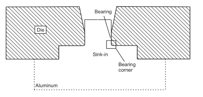

Figure: Die geometry around the bearing region
In this work, two limiting boundary conditions are considered: complete sticking and complete sliding.
A complete sticking condition is applied at the interface between the die face and aluminium. A complete sliding condition is applied at the interface between the bearing channel and aluminium.
The node located at the bearing corner, where the two interfaces meet, can have two different boundary conditions in the extrusion direction.
If the corner node is completely stuck, its movement is locked and the extrusion force is overestimated. If the node is allowed to slide freely in the extrusion direction, the extrusion force is underestimated and material-flow conservation can be violated.
An equivalent model is therefore required to represent the resistance to flow at the entrance of the bearing channel. The model must maintain material conservation while keeping the calculation time within a reasonable range.
Since the stress and strain at the bearing corner itself are not required, the corner can be represented using a relatively coarse mesh.
This chapter evaluates several approaches used in previous studies to model sharp corners and non-smooth boundaries. Two new approaches are then introduced.
The first represents the bearing corner with a single node and assigns it a conditional normal that maintains material-flow conservation. The corner radius is not explicitly included.
The second approach modifies the position of the corner node so that the effect of the corner radius can be represented.
The results are compared with a reference model containing a 0.5 mm radius and a friction coefficient of 0.4 between the die and aluminium. The mesh of the two-dimensional reference model is shown in Figure.
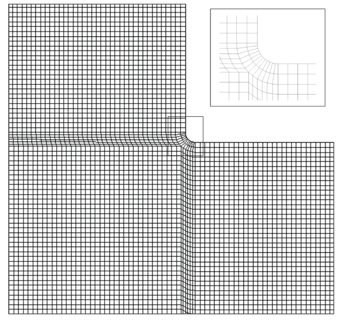

Figure: Mesh of the two-dimensional axisymmetric reference model
2.2 Previous Work
Different approaches have been proposed for dealing with flow around non-smooth boundaries.
One approach uses a sliding interface to solve fluid-structure interface problems. Each interface node is represented by two nodes, one on each surface. A local coordinate system is defined for each pair, with one direction tangent to the sliding interface and the other normal to it.
The two nodes are coupled in the normal direction but are free to slide tangentially. Their initial positions are assumed to be identical in the global coordinate system.
This approach is difficult to generalise because some knowledge of the surrounding flow is required to determine the orientation of the local coordinate system.
A similar concept has been applied to the bearing corner in aluminium extrusion using a three-node structure. Three nodes are created at the bearing corner and their degrees of freedom are connected so that the nodes move around the corner.
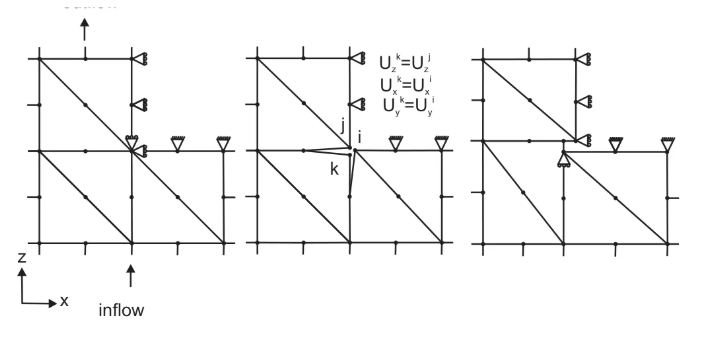

Figure: Three-node structure
With this approach, material flow is not always conserved.
The implementation also requires more preprocessing time, particularly for three-dimensional simulations. In addition, the lack of shear deformation at the element boundaries causes the extrusion force to be underestimated.
Another approach assigns a normal direction at a sharp corner when friction is present.
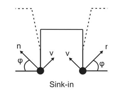

Figure: Normal at the entrance to the bearing channel
The normal is calculated as a weighted average of the normals of the element faces connected to the corner node. The weighting is based on the surface area of the elements connected to the corner.
Another method determines the weights so that the normal lies in a plane perpendicular to the average velocity through the thin region surrounding the corner.
In this approach, the normal is calculated iteratively, and its direction is not constant throughout the simulation. This increases the calculation time, while it is not clear whether material flow is fully conserved.
Another study examined the use of a chamfer to represent the sharp corner and assigned a normal at a specified angle.
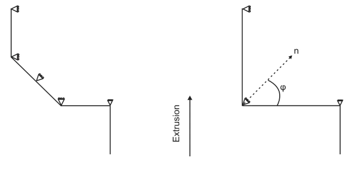

Figure: Modelling the sharp corner using a chamfer (left) and a normal (right)
For the chamfer, the two end nodes can move tangentially along the adjacent edges, while the middle node can move along the chamfer direction. For the normal representation, the node at which the normal is defined can move perpendicular to the normal.
Different normal angles ranging from 5° to 65° were investigated. The results showed that the chamfer and a normal with the optimum angle produced the best results in terms of extrusion force and streamline error.
Material conservation was not checked when the chamfer was used to construct the bearing corner.
When a normal was assigned to the bearing corner in a plane-strain finite element model, material conservation was examined for different normal angles. The condition was satisfied for the appropriate angle when a uniform mesh was used.
Using a chamfer introduces two additional parameters, its length and angle, which must be optimised during preprocessing. Since the chamfer must be represented by at least two elements, more elements are required than when the corner is represented by a normal.
By comparison, constructing a normal during preprocessing is relatively simple and direct.
The normal representation was therefore investigated further using two-dimensional models with uniform and non-uniform meshes and different element types. The element types included four-node plane-strain elements and four-node axisymmetric elements. Different extrusion ratios were also tested.
Relative error in exit velocity for different element types and extrusion ratios
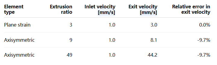

The results show that the selected normal works well for the plane-strain model but not for the axisymmetric model.
For the axisymmetric cases, the exit velocity error reaches approximately 10% at both extrusion ratios. This indicates a material-flow imbalance when the same normal is used in an axisymmetric finite element model.
Figure illustrates why material loss occurs in the axisymmetric model when the bearing-corner node moves perpendicular to the normal.
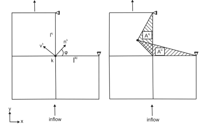

Figure: Inflow and outflow regions produced by movement perpendicular to the normal
For a uniform mesh, the two regions are equal in area. They can be regarded as the inflow and outflow regions.
In a plane-strain model, the inflow and outflow volumes are equal because their areas and thicknesses are identical.
In an axisymmetric model, however, the two volumes are different. Each volume depends on the area and the radius of its geometric centroid, according to Pappus’s centroid theorem.
Figure illustrates this relationship.
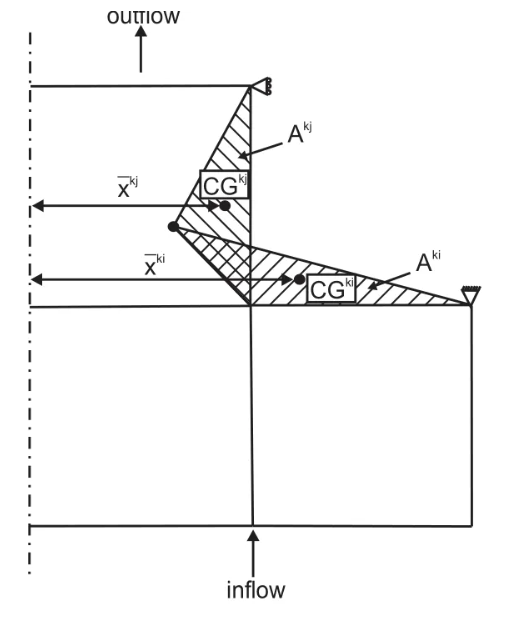

Figure: Pappus’s centroid theorem
The geometric centroid of the outflow region is located at a larger radius than the centroid of the inflow region. This explains the error in exit velocity obtained with axisymmetric elements.
The inflow region must therefore be increased so that the inflow and outflow volumes become equal. This can be achieved by increasing the angle of the normal.
For axisymmetric elements and a uniform mesh, the appropriate normal angle satisfies the material-conservation condition for this particular geometry.
When a filled die is used in an aluminium extrusion simulation, the element sizes around the bearing corner are not necessarily identical. The effect of this variation on the performance of the normal was therefore examined using axisymmetric elements.
The exit-velocity error and extrusion-force error were plotted against the element-size ratio. The errors are calculated relative to the exit velocity and extrusion force of the reference model.
The element-size ratio is defined as the downstream element size divided by the upstream element size.
The exit-velocity error disappears when the element-size ratio reaches 1.25. At this point, the inflow volume becomes larger than the outflow volume, compensating for the difference in the distances travelled by the centroids of the inflow and outflow regions.
The extrusion-force error changes with the element-size ratio.
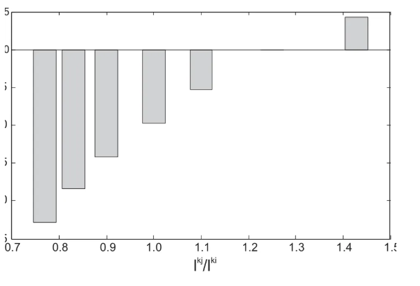

Figure: Exit-velocity error as a function of element-size ratio in the axisymmetric finite element model
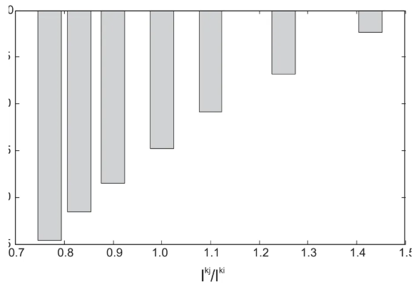

Figure: Extrusion-force error as a function of element-size ratio in the axisymmetric finite element model
These results show that the performance of the normal depends on the mesh. A new method is therefore needed to determine the normal direction.
2.3 Conditional Normal at the Sharp Corner
The direction of the normal assigned at the bearing corner is calculated so that the net volume change of the elements connected to the corner node is zero.
A displacement constraint is then applied to the bearing-corner node, allowing it to move only in the direction perpendicular to the conditional normal.
The concept is similar to the normal described previously, but the direction can be determined simply during preprocessing. The material-conservation condition is satisfied directly as a predefined constraint.
The normal direction is calculated from the areas of the element faces connected to the corner node and their corresponding unit normals.
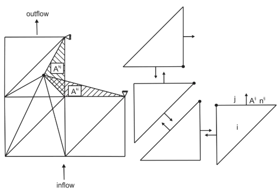

Figure: Elements surrounding the bearing corner
The preprocessing program loops through the bearing-corner nodes. For each corner node, it identifies all elements sharing that node and then determines the areas of the faces meeting at the node.
The resultant of these face-area vectors is then calculated to determine the equivalent boundary normal.
This implementation is simpler than approaches that require intersecting surface areas to be identified at the boundary. It can also be applied to different element types in both two- and three-dimensional models.
2.3.1 Representing the Conditional Normal in Aluminium Extrusion Simulations
There are two ways to represent the normal at the sharp corner.
The first is to define a linear constraint between the velocity components of the corner node. The constraint can be handled in a finite element program using several methods, including transformation matrices, Lagrange multipliers and the penalty method.
With the transformation-matrix approach, the constrained degree of freedom is condensed out. This requires rearranging the global stiffness matrix and performing matrix operations.
The transformation can be implemented at the global matrix level or at the element level. Its performance depends strongly on the efficiency of the implementation because many matrix operations are required.
The Lagrange multiplier method is not suitable because it increases the number of degrees of freedom. The penalty method is also unsuitable because it can introduce errors due to poor conditioning.
The second approach defines a local coordinate system at the corner node, rotated by the required angle, and suppresses movement in the normal direction,irection, as shown in Figure 2.11 as shown in Figure 2.11.
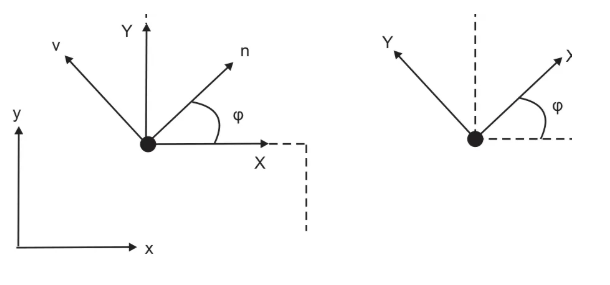
Figure: Representation of the normal using a local coordinate system
Both approaches were investigated. They produced the same results and required approximately the same calculation time.
2.4 Conditional Normal After Modifying the Geometry
The previous method does not account for the effect of the radius at the bearing corner. A new approach was therefore investigated in which the position of the corner node is changed before determining the normal direction.
The investigation began with a simple model uniformly discretised using four-node plane-strain elements.
The corner node can be positioned within a square region defined by the element size and corner radius. Different corner-node positions were investigated.
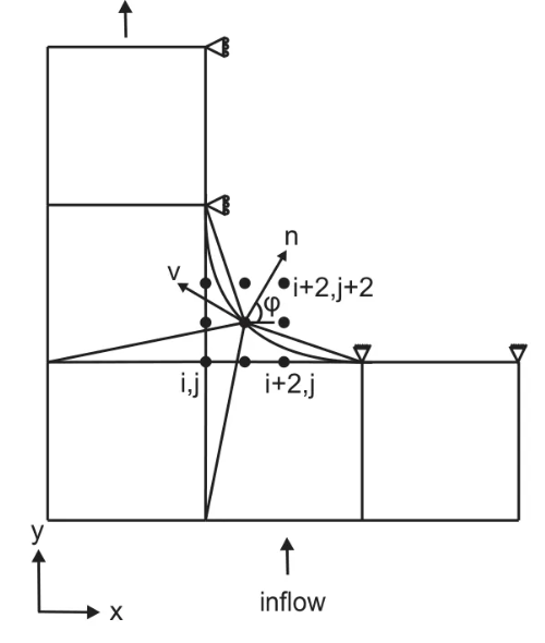

Figure: Possible positions of the bearing-corner node
As in the previous method, the relationship between the incremental material displacements at the corner node was determined for each position using.
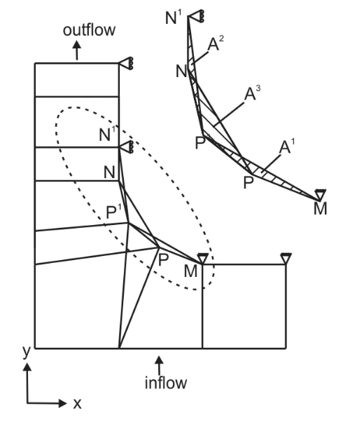

Figure: Construction of the constraint equation
Three regions are produced: one inflow region and two outflow regions.
Because one of these regions changes with the position of the corner node, the resulting relationship is nonlinear. The relationship was then linearised by assuming that the velocity at point N is known and equal to the ram velocity divided by the extrusion ratio.
The corresponding areas are defined by the triangular regions shown in the model.
At every corner-node position, extrusion force and material conservation were checked and compared with the reference model.
The extrusion force increases as the bearing-corner node moves radially. As shown , moving the corner node radially increases one of the regions. This increase must be compensated by increasing the horizontal component of the velocity at point P.
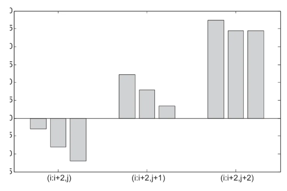

Figure: Extrusion-force error relative to the reference model
The linearised constraint equation does not conserve material flow at several of the investigated positions. The method was therefore not studied further.
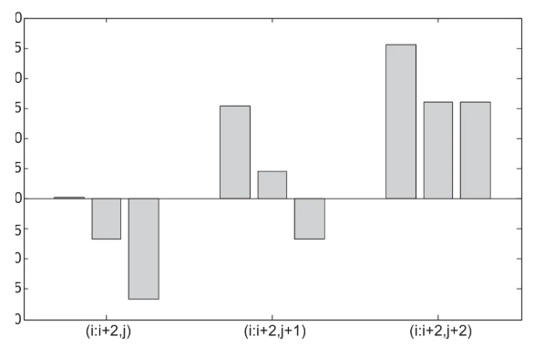

Figure: Exit-velocity error relative to the reference model
2.5 Three-Dimensional Example
Because tetrahedral elements are widely used in aluminium extrusion simulations, a three-dimensional example was used to evaluate different ways of constructing the bearing corner, including the conditional normal and the three-node structure.
The example simulates extrusion of a round bar with an extrusion ratio of 9 and a ram speed of 1 mm/s.
An isothermal Eulerian formulation was used.
For the boundary conditions, nodes in contact with the container and die face were assumed to stick, while nodes in contact with the bearing channel were free to slide in the extrusion direction.
The relative errors in extrusion force and exit velocity were calculated with respect to the reference model.
Exit velocity and extrusion-force errors for round-bar extrusion
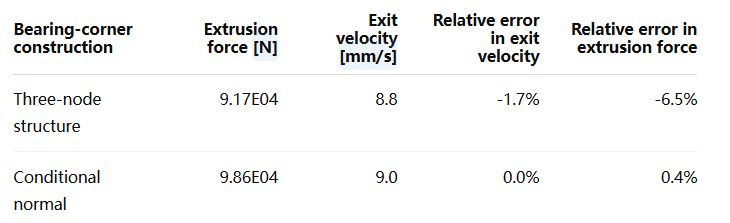

The results show that the three-node structure produces an exit-velocity error of approximately -1.7%, while the conditional normal gives the correct exit velocity.
This indicates that material conservation is not satisfied by the three-node structure.
The reason is that the degrees of freedom of the nodes representing the curved corner are connected in a Cartesian coordinate system.
A second example was therefore considered, this time modelling extrusion of a square bar at an extrusion ratio of 7 and a ram speed of 1 mm/s.
The simulation was carried out in a similar way to the previous example.
Exit velocity and extrusion force for square-bar extrusion


The table shows that material conservation is satisfied with the three-node structure for this particular geometry.
However, the extrusion force is underestimated because the element boundaries connected to the three-node structure do not allow sufficient shear deformation.
2.6 Summary and Conclusions
Several approaches for constructing sharp corners were examined in this chapter.
The normal-based approach was tested with different element types. The results showed that the selected normal works for two-dimensional models using uniformly distributed four-node plane-strain elements. With other two- and three-dimensional element types, the extrusion-force error may remain acceptable, but material conservation is not necessarily maintained.
The three-node structure has several disadvantages. It requires additional preprocessing time, underestimates extrusion force because of the lack of shear deformation at the element boundaries, and does not always conserve material flow. The problem is particularly relevant when profiles with curved surfaces are analysed.
The conditional normal avoids these problems. It does not require additional degrees of freedom and maintains material-flow conservation. It can be implemented with different two- and three-dimensional element types without adding significant preprocessing or solution time.
The approach that modifies the bearing-corner node position was found to be unsuitable because the resulting constraint equation contains nonlinear terms and the linearised form does not consistently conserve material flow.
3. Measuring Flat-Die Deflection
3.1 Introduction
Finite element simulations provide information about material flow and die deflection. Experimental measurements are required to validate the predicted die deformation.
This chapter describes an experimental setup used to measure die deflection and presents measurements of deflection, extrusion force and ram speed during the extrusion of more than one billet.
The experiment was carried out by the Boal Group.
3.2 Previous Measurement Methods
Measuring die deflection or pressure on the die face is challenging, particularly in an industrial extrusion environment. Several methods have been used to measure die-face pressure and tool deformation.
One study used semiconductor strain-gauge pressure sensors and a laser displacement sensor to measure pressure distribution on the die face and die deformation during extrusion of a 1050 aluminium bar. The experiment was carried out on a 400-ton vertical laboratory press.
The pressure sensor was inserted through a hole drilled through the die and its support so that the sensor was in direct contact with the metal. Die deformation was measured by monitoring the deflection of a rod attached to the die at a specified location using a laser displacement sensor.
Another approach determined die-face pressure from deformation measurements. A cylindrical flat steel capsule was inserted into the die face. The capsule was connected to the deformation-measurement system through a rod inserted into a hole drilled through the complete tool assembly.
A capacitive probe was also developed to measure pressure on the die face. This type of sensor was selected because of its small size and ability to operate at temperatures above 400°C.
The technique was successfully used on a laboratory vertical extrusion press to measure die-face pressure during round-bar and strip extrusion. However, the method was not completely successful when measuring die-face pressure during industrial extrusion of a U-shaped profile because of sensor failure.
Other studies used two laser displacement sensors based on laser triangulation to monitor the deflection of a die tongue during extrusion of two U-shaped profiles.
Three general approaches can be identified from these experiments.
The first measures die deflection by monitoring the deflection of a rod attached to the die face.
The second uses a laser displacement sensor to measure tongue deflection. This is similar to the first approach, but the laser beam replaces the rod.
The third uses sensors integrated into the die to measure deformation.
All of these approaches require modifications to the tool or the manufacture of a dedicated die capable of accommodating the sensors and their connections.
More importantly, they measure the absolute displacement of the die in the extrusion direction at a particular point rather than the relative displacement at the bearing.
The measured value therefore includes the translational deflection of the die as well as the movement of other tool components, such as the bolster, support plate and retaining ring.
This does not provide the true die deflection or information about bearing misalignment, even though bearing misalignment directly affects the dimensions of the extruded profile.
Additional measurements at other locations would therefore be required to determine the actual die deflection and bearing misalignment.
3.3 Experimental Setup
Because the experiment was carried out in an industrial environment, there was little freedom to modify the existing tool components.
A new setup was therefore developed in which a laser beam was directed onto a reflective surface mounted on the rear of the die.
The basic idea was to measure the angular deflection of the die tongue and use it to determine the relative displacement at the bearing.
With this arrangement, the relative displacement can be measured directly using a laser beam aimed at a single point.
3.3.1 Extrusion of the Profile
A U-shaped profile was selected for the experiment.
The die used to extrude this profile is subjected to both shear and bending stresses.
The profile was extruded on a 500-ton press with a 95 mm container diameter and an extrusion ratio of 11.658.
The billet was AA6060 aluminium containing 0.40% Si and 0.45% Mg.
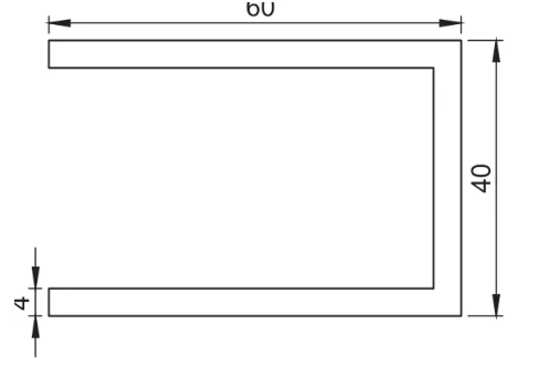

Figure: Profile geometry, dimensions in mm
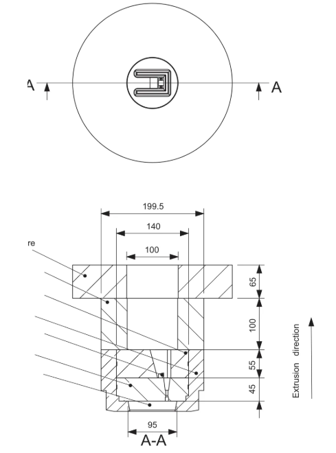

Figure : Tool assembly with reflector, dimensions in mm
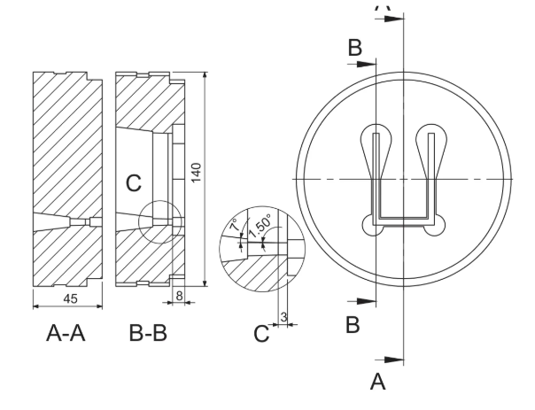

Figure: Die and sectional view
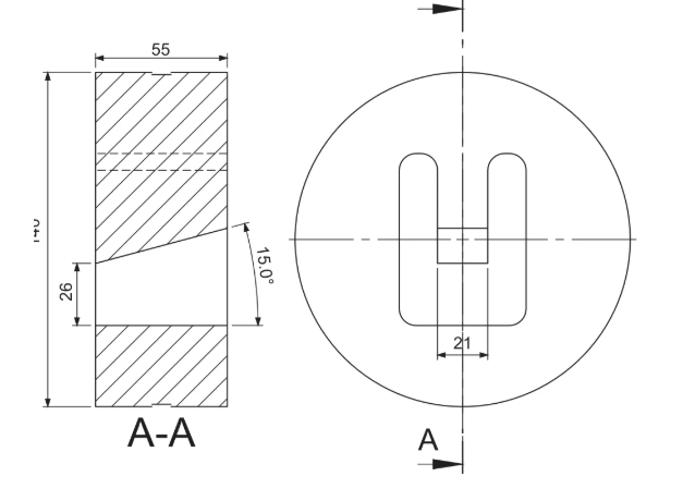

Figure: Front and sectional views of the bolster, dimensions in mm
The purpose of the experiment was to measure the angular deflection of the flat-die tongue.
The laser source was positioned outside the run-out table and away from the press because it operates at room temperature. It directed a laser beam toward a reflective surface, which reflected the beam onto a white screen.
A camera was positioned in front of the screen to record the movement of the reflected spot caused by die deflection.
The container pressure, seal pressure, ram speed and exit temperature were recorded simultaneously.
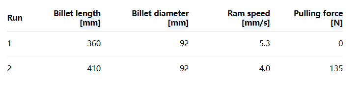
The experiment was performed twice using different settings to assess the results and their repeatability.
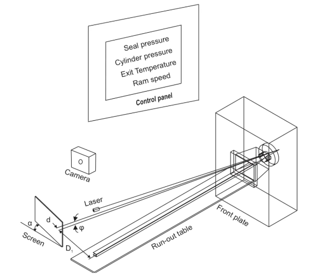

Figure: Experimental setup
Parameter settings for the two experimental runs

3.3.2 Determining Angular Deflection
The reflected laser beam was projected onto a screen with a white background and four reference points.
The reference points were used to calculate the movement of the reflected spot using a bilinear transformation.
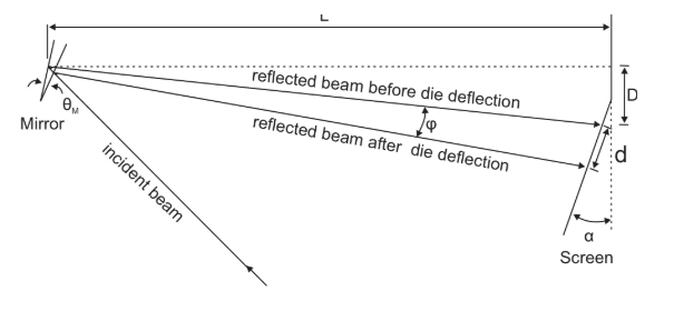

Figure: Schematic for calculating the angular deflection of the tongue
The screen remained fixed during the experiment.
The measurement errors associated with the screen dimensions were small enough to be neglected.
An error in calculating the displacement of the laser spot produces an error in the calculated tongue deflection. The estimated error in the spot displacement was taken as the radius of the laser spot on the screen, approximately 2.0 mm.
The resulting error in the calculated tongue angular deflection was approximately ±0.3 mrad.
3.3.3 Reflective Surface
Stainless steel was selected for the reflective surface because it can withstand high temperatures while maintaining its reflectivity during the experiment.
Because the laser source had to be positioned outside the run-out table, an inclined reflective surface was designed, as shown in Figure 3.7.
The inclination was selected so that both the incident and reflected beams remained within the visible range available through the opening in the retaining ring and at the tip of the tongue where the reflector was mounted.
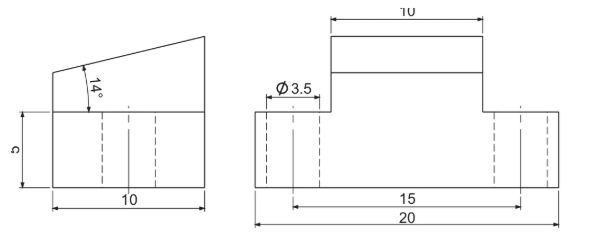

Figure: Front and side views of the reflective surface, dimensions in mm
An attempt was made to polish the small surface while maintaining adequate flatness, but this was unsuccessful.
The reflector was therefore manufactured by embedding a stainless-steel workpiece in phenolic resin, or Bakelite, and polishing a flat surface. The reflector was then removed by electrical discharge machining.
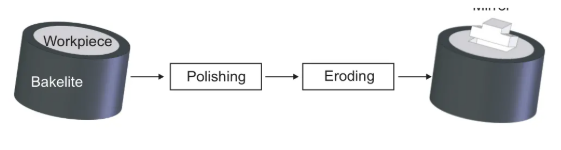

Figure: Manufacturing process for the reflective surface
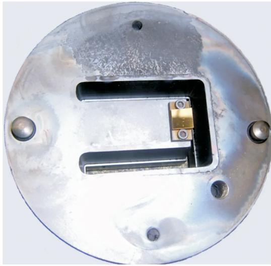

Figure: Reflector attached to the die tongue
3.3.4 Laser Source
The laser source was selected so that the diameter of the laser spot was smaller than the side length of the reflective surface.
The selected laser had the following specifications:
lGreen dot laser
lWavelength: 532 nm
lOutput power: 20 mW
lBeam divergence: 0.1 mrad
lAdjustable output diameter: 0.4–3.0 mm
3.3.5 Experimental Procedure
The experimental procedure was as follows:
1. Attach the reflector to the die.
2. Assemble the die, bolster, retaining ring and other tool components.
3. Place the tooling in the furnace and heat it to 460°C.
4. Position the laser source and screen within the visible area.
5. Position the camera.
6. Once the tooling reaches the required temperature, remove the die from the furnace and place it in the press.
7. Switch on the laser, aim it at the reflector and adjust the screen until the reflected spot can be captured. This must be done as quickly as possible to minimise tool cooling.
8. Switch on the camera and begin extrusion.
9. Record the actual positions of the laser source and screen.
3.3.6 Extrusion Cycle
Figure shows the changes in container pressure and seal pressure during the extrusion cycle.
Container pressure is the pressure applied to the ram to extrude the billet. Seal pressure indicates how tightly the container and tooling are locked together.
Based on the pressure history, the extrusion cycle can be divided into four stages:
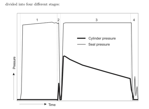

Figure: Stages of the extrusion cycle
1. The heated billet is loaded into the container.
2. The billet is upset and hot gas is released from the container during the burping stage.
3. The billet is extruded.
4. The butt end is sheared off.
The purpose of the burping stage is to remove hot gas from the container and prevent bubbles from forming.
If air remains trapped in the container during extrusion, it can become incorporated into the surface layer of the billet and travel along the material flow path. This can produce bubbles in the extruded profile, causing the profile to be rejected.
The optimum burping pressure is determined as the difference between the breakthrough pressure and the pressure at the end of the stroke.
It depends on billet length, ram speed and temperature.
The burping cycle accounts for approximately 10% of the idle cycle.
The idle cycle includes unloading the main cylinder, retracting the ram, opening the container, shearing the butt end, closing the container and advancing the ram to begin the next extrusion cycle.
3.4 Experimental Results
The two experimental runs were carried out on different dates using different setups to reduce the possibility of systematic errors.
3.4.1 Results from the First Run
Video recordings and process data from the extrusion of the first four billets were analysed.
After the billet was loaded into the container, the seal pressure increased to 210 bar to lock the container and tooling together.
The container pressure was then increased to 50 bar to upset the billet inside the 95 mm container. This pressure was referred to as the burping pressure.
During burping, the container pressure was reduced to zero and the container was moved backwards, allowing hot air to escape through the gap between the end of the container and the die face.
The container was then closed again and its pressure increased to 120 bar, after which extrusion of the billet began.
During extrusion, the container pressure decreased approximately exponentially as the friction area between the billet and container decreased.
The container pressure dropped by approximately 50 bar.
After the billet had been extruded, the container moved backwards and part of the hydraulic pressure was used to shear off the butt end.
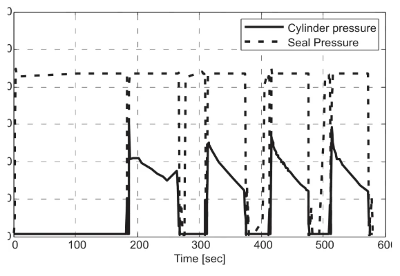

Figure: Pressure as a function of time during the first experimental run
The container-pressure curve for the first billet differs from those of the following billets because part of the first billet filled the die and the cavity between the die and retaining ring.
The extrusion force was calculated from the container pressure and container diameter.
The peaks in the extrusion-force curves for the third and fourth billets are higher than for the second billet because of cooling and changes in ram speed.
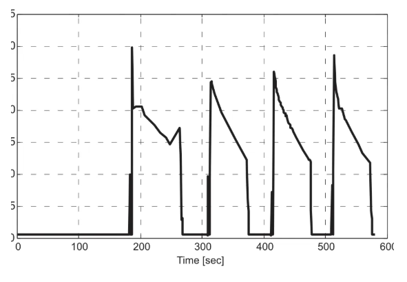

Figure: Extrusion force as a function of time during the first experimental run
The ram speed during the extrusion of the four billets is shown in Figure 3.13.
The nominal ram speed was 5.3 mm/s.
The extruded billet length was calculated by integrating ram speed over time.
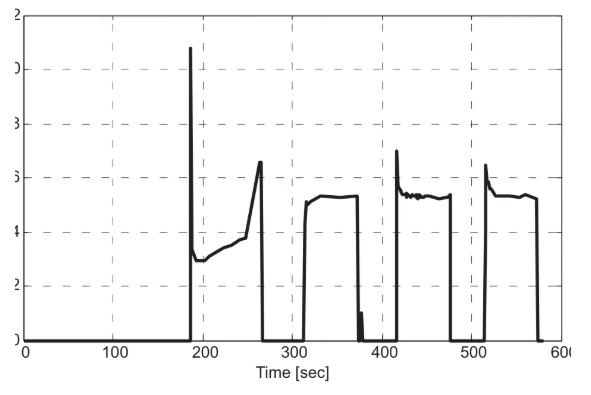

Figure: Ram speed as a function of time during the first experimental run
The movement of the reflected laser spot was determined from the video recording.
Figure 3.14 shows the distance travelled by the reflected spot during extrusion.
A program was developed using an image-processing toolbox to read the video and calculate the position of the spot throughout the extrusion process.
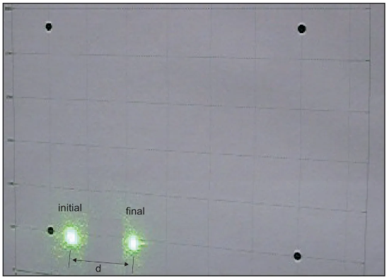

Figure: Initial and final positions of the reflected laser spot during extrusion in the first run
At the end of extrusion of the first billet and the subsequent billets, the tongue angular deflection reached approximately 8 mrad and 7 mrad, respectively.
The estimated measurement error was ±0.3 mrad.
The greater deflection during extrusion of the first billet was caused by the flexibility of the die.
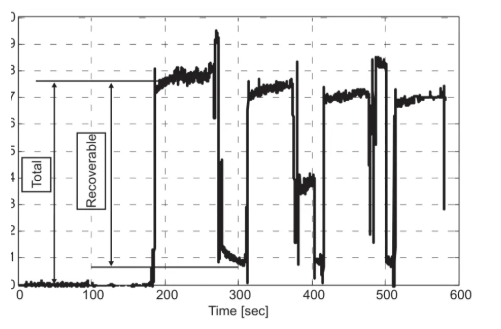

Figure: Tongue angular deflection as a function of time during the first experimental run
The angular deflection consists of a recoverable component and a permanent component.
The permanent component is the difference between the total angular deflection and the recoverable component. It was approximately 0.7 mrad.
The angular deflection also increased slightly during the extrusion of an individual billet. The increase was approximately 0.2 mrad.
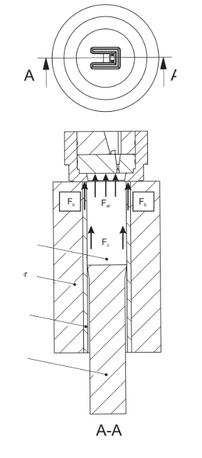

Figure: Loads acting on the tooling
This constraint force has been identified as a possible cause of the increase in angular deflection.
The force decreases during extrusion, and its effect on the angular deflection of the die tongue is examined further in the following analysis.
The die was inspected after the experiment, and a permanent deflection of approximately 0.03 mm was detected at the bearing.
This corresponds to an angular deflection of approximately 0.6 mrad in the tongue.
Finally, rigid-body movement of the tooling could be detected when the butt end was sheared off because the tooling was then free to move.
3.4.2 Results from the Second Run
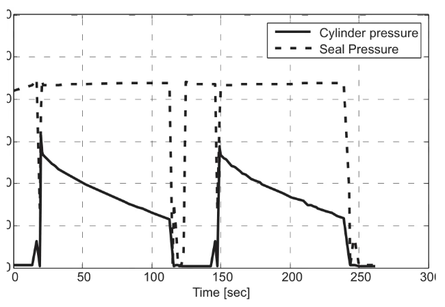

Figure:Pressure as a function of time during the second experimental run
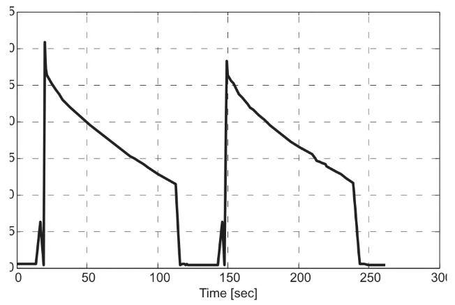

Figure: Extrusion force as a function of time during the second experimental run
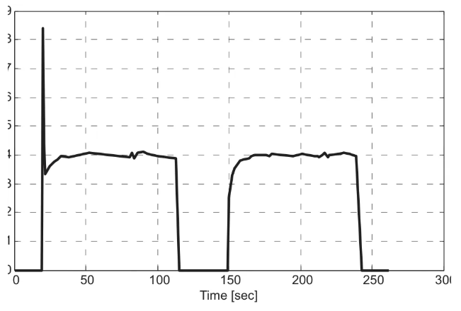

Figure: Ram speed as a function of time during the second experimental run
A breakthrough pressure of approximately 150 bar, higher than that of the first run because the billets used in the second run were longer.
As the friction area between the billet and container decreased, the pressure dropped by approximately 100 bar.
A nominal ram speed of approximately 4 mm/s, lower than that of the first run.
The tongue angular deflection reached approximately 5.8 mrad, with an estimated error of ±0.6 mrad.
The larger error in the second run was caused by the reduced reflectivity of the reflector after the die had been cleaned.
Inspection of the die after the second experimental run showed no additional permanent deflection.
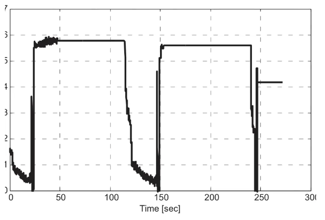

Figure: Tongue angular deflection as a function of time during the second experimental run
3.5 Summary and Conclusions
An experiment was carried out to measure the angular deflection of a die tongue during extrusion of a U-shaped profile.
The angular deflection was measured by directing a laser beam onto a reflective surface mounted on the die.
Two experimental runs were performed using different settings.
The experiment successfully measured the angular deflection of a flat-die tongue in an industrial environment. The modifications to the tooling were limited to a cut-out in the bolster and the attachment of the reflector, keeping the experimental setup relatively simple and practical.
The measured tongue angular deflection provides information about the relative displacement at the bearing, rather than the absolute displacement of the die. This makes it possible to monitor bearing misalignment.
The experiment produced realistic and repeatable results. It also showed that the die tongue undergoes a recoverable deflection during the extrusion of each billet.
Because the alignment between the tongue and die face was not checked before extrusion, however, it was not possible to determine whether the permanent deflection originated during extrusion of the first billet.
Post time: Sep-12-2026


